Stroke Prediction Model
Project in Progress
Preliminary code
Mass Effect Graph provided
Further Modeling and Accuracy needed
# Relevant Packages
library(pacman)
p_load(tidyverse, ggthemes, caret, mice, VIM, rpart, rpart.plot, effects, ggpubr, ROSE, pROC)
# Load Data
stroke <- read_csv("/Users/mohan/Desktop/Projects/26 Projects/Stroke Model/healthcare-dataset-stroke-data.csv") %>%
select(-c(id))
# Convert variables to appropriate data types
stroke <- stroke %>%
mutate(smoking_status = as.factor(smoking_status),
bmi = as.character(bmi),
bmi = gsub("[^0-9.]", "", bmi),
bmi = as.numeric(bmi),
work_type = as.factor(work_type),
hypertension = as.factor(hypertension),
Residence_type = as.factor(Residence_type),
stroke = as.factor(stroke),
ever_married = as.factor(ever_married),
heart_disease = as.factor(heart_disease),
gender = factor(gender, levels = c("Male", "Female")))
# Handle missing values in bmi
stroke <- stroke %>%
mutate(bmi = ifelse(is.na(bmi), mean(bmi, na.rm = TRUE), bmi))
# Data Partitioning
set.seed(123)
index <- createDataPartition(stroke$stroke, p = 0.7, list = FALSE)
train <- stroke[index, ]
test <- stroke[-index, ]
n_majority <- 1000 # Set the desired number of majority class samples
# Balancing the dataset
train_balanced <- ROSE(stroke ~ ., data = train, seed = 123, N = n_majority, p = 0.5)$data
train_balanced$stroke <- factor(train_balanced$stroke, levels = c("0", "1"))
# Model Building
dt_model <- rpart(stroke ~ ., data = train_balanced, method = "class")
# Predict on the test set
predictions <- predict(dt_model, test, type = "class")
# Convert test$stroke to factor with levels "0" and "1"
test$stroke <- factor(test$stroke, levels = c("0", "1"))
# Calculate AUC
roc <- pROC::roc(test$stroke, as.numeric(predictions))
# Imputation
imput <- mice(stroke, maxit = 0)
meth <- imput$method
predM <- imput$predictorMatrix
predM[, "bmi"] <- 0
set.seed(103)
imputed <- mice(stroke, method = meth, predictorMatrix = predM, m = 5)
stroke <- complete(imputed)
# Visualizations
# Gender
gender.dist <- tibble(gender = c("Female", "Male"),
total = as.numeric(table(stroke$gender))) %>%
mutate(gender.percent = round((total / sum(total) * 100))) %>%
ggplot(aes(x = "", y = gender.percent, fill = gender)) +
geom_bar(stat = "identity", color = "black") +
coord_polar("y", start = 0) +
theme_void() +
scale_fill_manual(values = c("#E0BBE4", "#FFDFD3", "#957DAD")) +
geom_text(aes(label = paste0(gender.percent, "%")))
gender.dist
# How many people in the dataset had a stroke
outcomes <- tibble(outcome = c("No Stroke", "Stroke"),
total = as.integer(table(stroke$stroke)))
outcome.dist <- outcomes %>%
mutate(stroke.percent = round((total / sum(total)) * 100)) %>%
mutate(ypos = cumsum(stroke.percent) - 0.5 * stroke.percent)
# Handle missing values in bmi
stroke <- stroke %>%
mutate(bmi = ifelse(is.na(bmi), mean(bmi, na.rm = TRUE), bmi))
# Data Partitioning
set.seed(123)
index <- createDataPartition(stroke$stroke, p = 0.7, list = FALSE)
train <- stroke[index, ]
test <- stroke[-index, ]
# Balancing the dataset
train_balanced <- ROSE(stroke ~ ., data = train, seed = 123, N = n_majority, p = 0.5)$data
train_balanced$stroke <- factor(train_balanced$stroke, levels = c("0", "1"))
# Model Building
dt_model <- rpart(stroke ~ ., data = train_balanced, method = "class")
# Predict on the test set
predictions <- predict(dt_model, test, type = "class")
# Convert test$stroke to factor with levels "0" and "1"
test$stroke <- factor(test$stroke, levels = c("0", "1"))
# Calculate AUC
roc <- pROC::roc(test$stroke, as.numeric(predictions))
# Imputation
imput <- mice(stroke, maxit = 0)
meth <- imput$method
predM <- imput$predictorMatrix
predM[, "bmi"] <- 0
set.seed(103)
imputed <- mice(stroke, method = meth, predictorMatrix = predM, m = 5)
stroke <- complete(imputed)
# Visualizations
# Gender
gender.dist <- tibble(gender = c("Female", "Male"),
total = as.numeric(table(stroke$gender))) %>%
mutate(gender.percent = round((total / sum(total) * 100))) %>%
ggplot(aes(x = "", y = gender.percent, fill = gender)) +
geom_bar(stat = "identity", color = "black") +
coord_polar("y", start = 0) +
theme_void() +
scale_fill_manual(values = c("#E0BBE4", "#FFDFD3", "#957DAD")) +
geom_text(aes(label = paste0(gender.percent, "%")))
gender.dist
# How many people in the dataset had a stroke
outcomes <- tibble(outcome = c("No Stroke", "Stroke"),
total = as.integer(table(stroke$stroke)))
outcome.dist <- outcomes %>%
mutate(stroke.percent = round((total / sum(total)) * 100)) %>%
mutate(ypos = cumsum(stroke.percent) - 0.5 * stroke.percent)
outcome.dist
# Feature Engineering
# Age Binning
stroke$age_group <- cut(stroke$age, breaks = c(0, 18, 40, 60, max(stroke$age)), labels = c("0-18", "19-40", "41-60", "61+"))
# BMI Category
stroke$bmi_category <- cut(stroke$bmi, breaks = c(0, 18.5, 25, 30, max(stroke$bmi)),
labels = c("Underweight", "Normal", "Overweight", "Obese"))
stroke$bmi <- as.numeric(gsub("[^0-9.]", "", trimws(stroke$bmi)))
# Data Visualization
# Age Group Distribution
age_group_dist <- stroke %>%
group_by(age_group) %>%
summarize(total = n()) %>%
mutate(age_group_percent = round((total / sum(total)) * 100)) %>%
ggplot(aes(x = age_group, y = age_group_percent, fill = age_group)) +
geom_bar(stat = "identity", color = "black") +
theme_minimal() +
xlab("Age Group") +
ylab("Percentage") +
ggtitle("Distribution by Age Group") +
geom_text(aes(label = paste0(age_group_percent, "%")), vjust = -0.5) +
theme(legend.position = "none")
age_group_dist
# BMI Category Distribution
bmi_category_dist <- stroke %>%
group_by(bmi_category) %>%
summarize(total = n()) %>%
mutate(bmi_category_percent = round((total / sum(total)) * 100)) %>%
ggplot(aes(x = bmi_category, y = bmi_category_percent, fill = bmi_category)) +
geom_bar(stat = "identity", color = "black") +
theme_minimal() +
xlab("BMI Category") +
ylab("Percentage") +
ggtitle("Distribution by BMI Category") +
geom_text(aes(label = paste0(bmi_category_percent, "%")), vjust = -0.5) +
theme(legend.position = "none")
bmi_category_dist
# Model Evaluation
# Confusion Matrix
confusion_matrix <- confusionMatrix(predictions, test$stroke)
confusion_matrix
# Accuracy
accuracy <- confusion_matrix$overall["Accuracy"]
accuracy
# AUC
auc <- roc$auc
auc
# Sensitivity and Specificity
sensitivity <- confusion_matrix$byClass["Sensitivity"]
specificity <- confusion_matrix$byClass["Specificity"]
sensitivity
specificity
library(ggplot2)
library(gridExtra)
# Demographics based on all categories
gender_plot <- ggplot(stroke, aes(x = gender)) +
geom_bar() +
labs(x = "Gender", y = "Count") +
ggtitle("Distribution of Gender")
age_plot <- ggplot(stroke, aes(x = age)) +
geom_histogram() +
labs(x = "Age", y = "Count") +
ggtitle("Distribution of Age")
ever_married_plot <- ggplot(stroke, aes(x = ever_married)) +
geom_bar() +
labs(x = "Marital Status", y = "Count") +
ggtitle("Distribution of Marital Status")
work_type_plot <- ggplot(stroke, aes(x = work_type)) +
geom_bar() +
labs(x = "Work Type", y = "Count") +
ggtitle("Distribution of Work Type")
residence_type_plot <- ggplot(stroke, aes(x = Residence_type)) +
geom_bar() +
labs(x = "Residence Type", y = "Count") +
ggtitle("Distribution of Residence Type")
# Demographics for those who had a stroke
stroke_subset <- subset(stroke, stroke == 1)
gender_stroke_plot <- ggplot(stroke_subset, aes(x = gender)) +
geom_bar() +
labs(x = "Gender", y = "Count") +
ggtitle("Distribution of Gender for Stroke Cases")
age_stroke_plot <- ggplot(stroke_subset, aes(x = age)) +
geom_histogram() +
labs(x = "Age", y = "Count") +
ggtitle("Distribution of Age for Stroke Cases")
ever_married_stroke_plot <- ggplot(stroke_subset, aes(x = ever_married)) +
geom_bar() +
labs(x = "Marital Status", y = "Count") +
ggtitle("Distribution of Marital Status for Stroke Cases")
work_type_stroke_plot <- ggplot(stroke_subset, aes(x = work_type)) +
geom_bar() +
labs(x = "Work Type", y = "Count") +
ggtitle("Distribution of Work Type for Stroke Cases")
residence_type_stroke_plot <- ggplot(stroke_subset, aes(x = Residence_type)) +
geom_bar() +
labs(x = "Residence Type", y = "Count") +
ggtitle("Distribution of Residence Type for Stroke Cases")
# Clinical metrics
hypertension_plot <- ggplot(stroke, aes(x = hypertension)) +
geom_bar() +
labs(x = "Hypertension", y = "Count") +
ggtitle("Distribution of Hypertension")
heart_disease_plot <- ggplot(stroke, aes(x = heart_disease)) +
geom_bar() +
labs(x = "Heart Disease", y = "Count") +
ggtitle("Distribution of Heart Disease")
bmi_plot <- ggplot(stroke, aes(x = bmi)) +
geom_histogram() +
labs(x = "BMI", y = "Count") +
ggtitle("Distribution of BMI")
glucose_level_plot <- ggplot(stroke, aes(x = avg_glucose_level)) +
geom_histogram() +
labs(x = "Average Glucose Level", y = "Count") +
ggtitle("Distribution of Average Glucose Level")
# First grid arrangement
grid_arrange_1 <- function(...) {
grid.arrange(..., ncol = 2)
}
# Second grid arrangement
grid_arrange_2 <- function(...) {
grid.arrange(..., ncol = 2)
}
# Arrange and display the graphs
grid_arrange_1(
gender_plot, age_plot,
ever_married_plot, work_type_plot,
residence_type_plot, gender_stroke_plot,
age_stroke_plot, ever_married_stroke_plot,
nrow = 4
)
grid_arrange_2(
work_type_stroke_plot, residence_type_stroke_plot,
hypertension_plot, heart_disease_plot,
bmi_plot, glucose_level_plot,
nrow = 4
)
library(caret)
library(ROSE)
library(rpart.plot)
set.seed(123)
# Split the data into training and testing sets
index <- createDataPartition(stroke$stroke, p = 0.8, list = FALSE)
train_data <- stroke[index, ]
test_data <- stroke[-index, ]
# Using ROSE for synthetic data generation (due to imbalanced nature of outcomes)
oversampled_data <- ovun.sample(stroke ~ ., data = train_data, method = "over", N = 2 * nrow(train_data), seed = 123)$data
# Build the binary tree model
tree_model <- rpart(stroke ~ .,
data = oversampled_data, method = "class", control = rpart.control(cp = 0.01))
# Make predictions on the test data
predictions <- predict(tree_model, newdata = test_data, type = "prob")
# Adjust classification threshold for sensitivity improvement
threshold <- 0.
predicted_class <- as.numeric(predictions[, 2] > threshold)
# Calculate misclassification rate
misclassification_rate <- mean(predictions != test_data$stroke)
# Print the binary tree
printcp(tree_model)
# Plot the binary tree
rpart.plot(tree_model)
# Evaluate variable importance
var_importance <- varImp(tree_model, scale = FALSE)
# View variable importance
print(var_importance)
# Predict on test data
test_pred <- predict(tree_model, newdata = test_data, type = "class")
# Evaluate the model
confusion_matrix <- table(test_pred, test_data$stroke)
accuracy <- sum(diag(confusion_matrix)) / sum(confusion_matrix)
misclassification_rate <- 1 - accuracy
# Calculate sensitivity, specificity, and F1 score
sensitivity <- confusion_matrix[2, 2] / sum(confusion_matrix[2, ])
specificity <- confusion_matrix[1, 1] / sum(confusion_matrix[1, ])
precision <- confusion_matrix[2, 2] / sum(confusion_matrix[, 2])
f1_score <- 2 * (precision * sensitivity) / (precision + sensitivity)
# View the confusion matrix, misclassification rate, sensitivity, specificity, and F1 score
print(confusion_matrix)
print(paste("Misclassification Rate:", round(misclassification_rate, 4)))
print(paste("Sensitivity:", round(sensitivity, 4)))
print(paste("Specificity:", round(specificity, 4)))
print(paste("F1 Score:", round(f1_score, 4)))
library(caret)
library(ROSE)
library(randomForest)
set.seed(123)
# Split the data into training and testing sets
index <- createDataPartition(stroke$stroke, p = 0.8, list = FALSE)
train_data <- stroke[index, ]
test_data <- stroke[-index, ]
# Using ROSE for synthetic data generation (due to imbalanced nature of outcomes)
oversampled_data <- ovun.sample(stroke ~ ., data = train_data, method = "over", N = 2 * nrow(train_data), seed = 123)$data
# Build the Random Forest model
rf_model <- randomForest(stroke ~ ., data = oversampled_data, importance = TRUE)
# Make predictions on the test data
predictions <- predict(rf_model, newdata = test_data)
# Evaluate the model
confusion_matrix <- table(predictions, test_data$stroke)
accuracy <- sum(diag(confusion_matrix)) / sum(confusion_matrix)
misclassification_rate <- 1 - accuracy
sensitivity <- confusion_matrix[2, 2] / sum(confusion_matrix[2, ])
specificity <- confusion_matrix[1, 1] / sum(confusion_matrix[1, ])
# Calculate the F1 score manually
precision <- confusion_matrix[2, 2] / sum(confusion_matrix[, 2])
recall <- sensitivity
f1_score <- 2 * (precision * recall) / (precision + recall)
# View the confusion matrix, performance metrics, and F1 score
print(confusion_matrix)
cat("Misclassification Rate:", misclassification_rate, "\n")
cat("Sensitivity:", sensitivity, "\n")
cat("Specificity:", specificity, "\n")
cat("F1 Score:", f1_score, "\n")
# Apply preprocessing to the training data
preprocessed_data <- preProcess(train_data, method = c("center", "scale"))
# Transform the training data using the preprocessed data
train_data_transformed <- predict(preprocessed_data, train_data)
# Train the logistic regression model
logistic_model <- glm(stroke ~ ., data = train_data_transformed, family = binomial())
# View the summary of the model
summary(logistic_model)
# Apply the same preprocessing to the test data
test_data_transformed <- predict(preprocessed_data, test_data)
# Make predictions on the test data
pred <- predict(logistic_model, newdata = test_data_transformed, type = "response")
# Convert predicted probabilities to class labels
pred_class <- ifelse(pred > 0.5, 1, 0)
# Evaluate the model performance using accuracy
accuracy <- mean(pred_class == test_data_transformed$stroke)
print(accuracy)
# Calculate true positives, true negatives, false positives, and false negatives
tp <- sum(pred_class == 1 & test_data_transformed$stroke == 1)
tn <- sum(pred_class == 0 & test_data_transformed$stroke == 0)
fp <- sum(pred_class == 1 & test_data_transformed$stroke == 0)
fn <- sum(pred_class == 0 & test_data_transformed$stroke == 1)
# Calculate sensitivity (true positive rate)
sensitivity <- tp / (tp + fn)
# Calculate specificity (true negative rate)
specificity <- tn / (tn + fp)
# Calculate precision, recall, and F1 score
precision <- tp / (tp + fp)
precision[is.nan(precision)] <- 0 # Set precision to 0 if NaN
recall <- sensitivity
recall[is.nan(recall)] <- 0 # Set recall to 0 if NaN
f1_score <- ifelse((precision + recall) > 0, 2 * (precision * recall) / (precision + recall), 0)
# Calculate misclassification rate
misclassification_rate <- mean(pred_class != test_data_transformed$stroke)
# Print the results
cat("Misclassification Rate:", misclassification_rate, "\n")
cat("Sensitivity:", sensitivity, "\n")
cat("Specificity:", specificity, "\n")
cat("F1 Score:", f1_score, "\n")
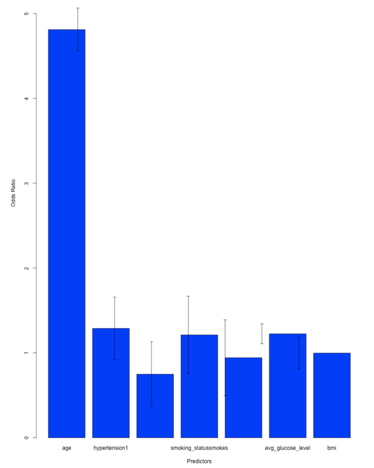
# Fit the logistic regression model
model <- glm(stroke ~ age + hypertension + smoking_status + avg_glucose_level + bmi,
data = train_data_transformed, family = binomial())
# Get the coefficients
coefficients <- coef(model)
predictors <- names(coefficients)[-1] # Exclude the intercept
# Compute the odds ratios
odds_ratios <- exp(coefficients[-1])
names(odds_ratios) <- predictors
# Create a bar plot of the odds ratios
barplot(odds_ratios, main = "Effects of Factors on Stroke Risk",
xlab = "Predictors", ylab = "Odds Ratio", col = "blue", ylim = c(0, max(odds_ratios) * 1.2))
# Add error bars indicating the 95% confidence intervals
errors <- coef(summary(model))[-1, "Std. Error"]
arrows(x0 = 1:length(predictors), y0 = odds_ratios - 1.96 * errors,
x1 = 1:length(predictors), y1 = odds_ratios + 1.96 * errors,
angle = 90, code = 3, length = 0.05)